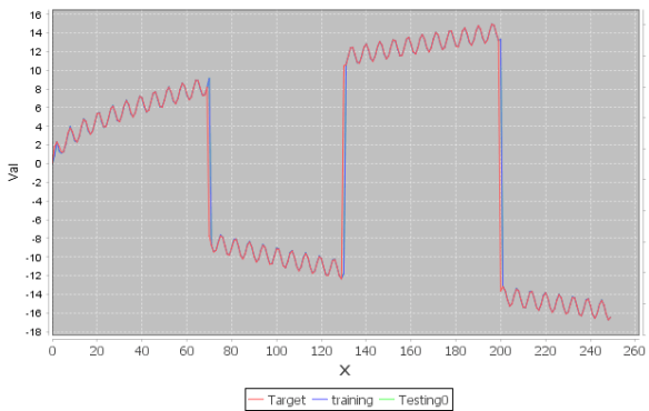
In the last several posts, I used genetic programming (GP) to model time series by fitting an equation to observed data. The resultant equation was used to predict unseen data points. In this post, I discuss applying similar techniques to market investment decisions.

In their introductory textbook, Poli et al. list characteristics of problems that are well suited for GP. These characteristics are:

The interrelationships among the relevant variables is unknown or poorly understood (or where it is suspected that the current understanding may possibly be wrong).

Finding the size and shape of the ultimate solution is a major part of the problem.

Significant amounts of test data are available in computer-readable form.

There are good simulators to test the performance of tentative solutions to a problem, but poor methods to directly obtain good solutions.

Conventional mathematical analysis does not, or cannot, provide analytic solutions

An approximate solution is acceptable (or is the only result that is ever likely to be obtained)

Small improvements in performance are routinely measured (or easily measurable) and highly prized.

(Poli et al., 2008, pp.11-13)

Without much further explanation, it is evident to me that all these characteristics are apt descriptions of the problem of stock market prediction

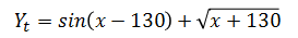
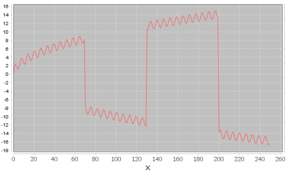
Continuing with the equation fitting approach, we could attempt to model an equation describing a financial time series such as the S&P 500 Index. Assume we could determine an equation of the form

Today’s close = f (today’s date, historical prices)

that closely fits past price history. To apply this equation to investment decisions, we would need to determine the closing price for the following market date and decide whether to be invested or not for that day. To make predictions in this manner, we would need an almost omniscient knowledge of the exact path of the market. Achieving this aim is unlikely for many reasons, one being the large random factors influencing any day to day market move. To avoid the impact of day to day fluctuations, we might make predictions further out in the future, but how far?  One option is to train the predictors using a criterion such as “will the target series gain X% in M days”, where X and M are user supplied values (Kampouridis & Tsang, 2010).  While fitting an equation is a form of symbolic regression, this approach is a form of supervised learning.  At any historical point, we know for certain whether an investment at that point would satisfy the target requirements of a specific future percentage gain, without the need to identify a specific equation. The resultant program would return a Boolean value instead of the numeric value used in our prior time series experiments.

An alternative GP approach looks at the broader question of whether to be in or out of the market at any point in time. Instead of a specific target return criterion, this approach simply asks, “find me the program that makes the most money” and evolves a program that yields the highest profit over the investment horizon. This is a form of unsupervised learning, as we are not providing the training algorithm the correct decision at any point in time.

In the following experiment, I will use GP to evolve a population of computer programs that return a Boolean (true or false) value determining whether to be fully invested or fully out of the market. The S&P 500 is used as the target investment. The evolutionary operations decide the applicable criteria for investment decision. Multiple fitness factors can be considered, such as the Sharpe ratio, maximum drawdown, etc., though this experiment will only look at investment return as the fitness criteria. This approach illustrates the flexibility of GP and is the approach is currently used in Evolutionary Signals.

Recall, GP evolves a population of computer programs over a set number of training generations to solve a targeted problem. After training, the best performing program is taken as the solution to the target problem. In this case, the best performing program will be use to make investment decisions.

Several training approaches are possible. These are:

1. Train->Predict
2. Train->Test->Predict

In the first approach, we run a fixed number of training generations on the GP population. At the end of the training phase, we use the best program for prediction.  A problem with this approach is that the chosen prediction program may greatly overfit the training data and not be very applicable to out of sample data seen in ongoing prediction. Periodic retraining can somewhat ameliorate this issue.

A better training approach is to incorporate an out of sample testing phase. Again, we run GP for a set number of training generations. A new phase is added where the best performing program from the training phase is used to make predictions on a new set of test data. For time series, the test data needs to occur chronologically after the training data to avoid data snooping. GP runs this train-test cycle several times with the best program from each phase recorded. The best performing program over the set of testing phases is chosen for initial prediction. This approach takes more time to train, however.

In both approaches, training will generally continue during the ongoing prediction phase. Neither approach avoids the possibility that the training and testing periods are vastly different from data seen in the actual prediction periods. Again, periodic retraining, plus other techniques dealing with regime change, may help avoid this problem. Regime change approaches will be discussed on a future post. This issue is also addressed in my PhD dissertation.

While a nearly limitless number of predictor series are available, this experiment will use the S&P 500 daily close and volume history. Transaction costs will be ignored as will returns when out of the market. These are two factors traditionally used in technical analysis (as they were the only factors available back in the day, before company fundamental became widely available).

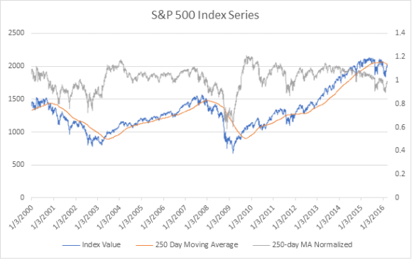
Most machine learning tasks require data to be normalized. Normalization smooths out discrepancies in scale within and between series. For example, comparing the units of S&P 500 price (thousands) to volume (billions) could greatly skew the results. In this experiment, I will apply mean normalization to both predictor series by dividing each price or volume value by the corresponding 250-day moving average. This operation transforms both series to a similar scale, fluctuating around 1. The following chart shows the target and normalized price series for the period considered in the experiment.

There are hundreds of technical indicators available (see  Investopedia for a nice list) that could be incorporated into the GP algorithm, in addition to core the mathematical functions that were used in the prior time series experiments.  This experiment will include several of the most common including:

• Momentum- compare the current value to a recent average (Ex. Buy if current price exceeds the 30-day moving average)
• Breakout- compare the current value to a recent minimum/maximum (Ex. Buy if current price risen by 2% over minimum price last 30 days)

There is a tradeoff between using high level packaged indicators, such as those listed on Investopedia, and lower level functions. Ideally, using lower level functions will discover new and novel indicators. Using higher level functions could yield better performance as these are technical indicators with known utility, but most of these are widely followed and it may be more difficult to act on signals in a timely manner.

The follow primitives will be used in the experiment:

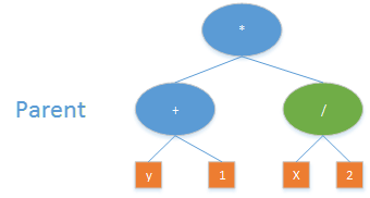
From this raw material, GP will evolve a population of programs (Boolean expressions) determining whether to invest or not at any point in time. A sample program we hope might evolve is:

(> (OffsetValue SP500 1) (MovingAverage SP500 30)

The expression states: invest if the prior day’s value of the S&P 500 index is above its 30-day moving average.

In the next post, I will provide the results of this prediction experiment.

References

Kampouridis, M., & Tsang, E. (2010). EDDIE for Investment Opportunities Forecasting: Extending the Search Space of the GP. In 2010 IEEE Conference on Evolutionary Computation (CEC) (pp. 1–8). IEEE.

Poli, R., Langdon, W. B., McPhee, N. F., & Koza, J. R. (2008). A field guide to genetic programming. Lulu. com.

In prior posts, I showed that genetic programming could be used to fit an expression to a set of experimental data. This technique is know as symbolic regression and is used to model the underlying data generating process (DGP) describing observed data points. A series that was easily modeled is show again below

The underlying DGP is described by the equation :

In that experiment, genetic programming did a good job of approximating this series, with a final mean error of 0.012.

But what happens if the DGP changes, either abruptly or gradually, over time? Financial series are known to exhibit this behavior. For example, the following chart of the S&P 500 before and after the financial crisis in 2008. The underlying factors before and after the crash and during the subsequent recovery are likely quite different.

S&P 500 index close price during the stock market crash of 2008 (Yahoo, 2013)

An example synthetic (made up) series that exhibits structure breaks, or regime change, is the following:

This series is represented by the equation:

Taken separately as two (or possibly four) individual series, GP would easily find the correct solution to each. But without a way to break the series up, GP does not perform very well. Using the same parameters as in the prior experiment, GP finishes the run with an average error of 1.71, compared with an average error of .01 for the (slightly more complicated) series in the prior experiment.

The final regression achieved is shown in the following diagram:

You can view the log of the run :

[Symbolic regression with regime change log.txt].

The video is shown below.

One easy way to improve this situation is to add autoregressive and logical functions to the primitive set. By autoregressive, I mean functions that make use of prior series values. Chaotic series are determined by such functions, but this series is not chaotic. However, adding such functions can yield much better predictions. As we know the actual DGP does not include an autoregressive term, the use of such functions will likely not indicate the actual DGP, but only an approximation. Additional logical functions are included to enable decisions that could potentially model underlying regime switching.

A risk in including autoregressive functions is that the prediction can converge early to a random walk prediction, where the predicted value is simply the prior value. One way to avoid this is to not allow expressions that evaluate to the prior value. While this may be cheating a bit for this series, autocorrelation functions are requirements for chaotic series and likely required for financial series.

The following experiment adds the following three functions to the primitive set:

• PeriodMin – minimum x value within a given prior period
• PeriodMax – maximum x value within a given prior period
• OffsetValue – value of x a given period ago.

For these three functions, the offset periods are determined through evolutionary operations.

The following logical expressions are also added:

• And  – logical And
• Not  – logical negation
• GT  – logical greater than
• LT  – logical less than
• ifElseBoolean – if else with Boolean parameters
• ifElseNumeric –if else with numeric parameters

The following run uses the same parameters as the prior run along with the inclusion of the additional primitives.

The log of the run is here:

[Symbolic regression with regime change and autoregressive functions log.txt]

and a video of the run is shown below.:

Notice the prediction immediately converges on a somewhat trivial prediction but adjusts and improves over time. The diagram below shows the results after one generation. The function shown is the equivalent of y(t)=y(t-1) +1.

The final result does a bit better, with an average error of 0.31, and is shown in the diagram below. Still, the result is not as good as what can be achieved on similar series that don’t contain structural breaks.

An analyst looking at this series might notice that it is broken up into either two series or four similar segments. Therefore, he might choose to run different models on each section and take each prediction individually. In fact, this is often how regime change is handled when modeling financial series*. However, forcing the analyst to choose the appropriate time window for analysis limits the potential automated solutions (Wagner et al., 2007. P.2).

An alternative approach that I developed in my PhD dissertation automatically infers regime boundaries and allows the development of distinct solutions for each regime. Using this technique, the run converges to the exact solution (ignoring some rounding errors) after 26 generations. The final (correct) solution is shown below.

The black line shows the inferred regimes, as indicated by the right vertical axis. In this approach, different expressions are automatically generated for different regimes. Regime boundaries are determined through typical evolutionary operations.

Here is the log for this run

[Symbolic regression with regime change and automatically defined templates log.txt.

A video of the run is shown below.

I will discuss this technique, which I named “automatically defined templates”, further in future blogs. For now, you can see my PhD dissertation for additional information.

* Two econometric methods, threshold autoregressive model and the Markov regime switching model, consider regime change. Both approaches break the time series into two or more separate series, one for each regime, and apply traditional modeling techniques, such as ARMA, to each independently.

References:

Wagner, N., Michalewicz, Z., Khouja, M., & McGregor, R. R. (2007). Time Series Forecasting for Dynamic Environments: The DyFor Genetic Program Model. IEEE Transactions on Evolutionary Computation, 11(4), 433–452. doi:10.1109/TEVC.2006.882430

Yahoo. (2013). Yahoo Finance. Retrieved from http://finance.yahoo.com/

In the last part of this series introducing genetic programming (GP), I described a simple experiment in symbolic regression. In that experiment, a formula was discovered based on data observations. This formula, modeling the underlying data generating process (DGP) can be used for predicting out of sample values. As the DGP was quite simple, the formula was consistently discovered in a handful of generations.

An  example of a slightly more complicated DGP is shown below:

This series is described by the formula:

To model the DGP for this series, I set up a GP run the perform symbolic regression using the following parameters:

A video of the run is shown below. The red series is the target equation. The blue series is the best fit after each generation. If all goes well, the blue series will eventually converge to the red series.

You can view the log of the run [Symbolic Regression Log 3.txt].

While the mean error is not zero—the model is not exact—GP does a reasonable job at approximating the target series, with a final mean error of 0.011952. The mean error is the average error in each of 100 points of the predicted x,y value compared to the known x,y value.

As I did in the prior blog post, I will prove that the GP methodology works. In the second experiment, I set the tournament size to 1, essentially eliminating the “fittest” from survival of the fittest. Elitism is still used, so any fit individual uncovered through mutation and crossover will be retrained. However, these mutations and crossovers do not necessarily use fitter individuals.

This run does a much worse job then the first example, giving a mean square error of  0.70398.

A video of the run is shown below. Very little progress is made over the 100 generation run.

You can view the log of the run [Symbolic Regression Log 4.txt].

I executed ten runs comparing the modeling using tournament sizes 1 and 4. The average mean error over each generation is shown in the chart below.

In the real world, series we choose to model are not generally as simple as the target series described above. An example of such series are chaotic series.  An example is the following

The equation for this series is:

Chaotic series are generally described as series that appear random but a highly dependent on their initial conditions, in this case, Y(0)=0.9. A different initial value might yield a series that looks entirely different. As these series are actually deterministic, they can therefore be accurately modeled. However, in reality,  these series are very hard to model and predict, as even a small error in predicted initial value will lead to a much larger error in overall accuracy.

In the first experiment on this series, I use the parameters below, which are essentially the same as what was used in the first experiment.

The results are not very good. The mean error of this run is 0.21638 . GP has an extremely hard time modeling this chaotic series as it lacks sufficiency, meaning the input parameters are not sufficient to find the actual solution.

A video of the run is shown below.

You can view the log of the run [Symbolic Regression Log 5.txt].

Looking back at the formula describing the DGP, we can see that the current values are dependent on prior series values. This phenomenon is typical with chaotic series. By including two additional terminals providing the prior two values of the series, a much better approximation is found.

This run achieved a mean error of 0.002874, much better than the initial run.

A video of the run is shown below.

You can view the log of the run [Symbolic Regression Log 6.txt]

I executed the second set of runs ten times, with and without the additional two autoregressive terminals. The results are shown in the following figure.

The results of these experiments indicate that while GP is highly parameter dependent, as long as sufficiency is satisfied, results will tend to converge towards the correct or optimal solution.

As these demos did not take very long to run, it is certainly possible to get better results by using larger population sizes or running for more generations.  In practice, we would certainly do this. However, for series with continually changing DGP (think stocks), increasing these parameters could lead to over-fitting or at least difficulty in reacting to such changes. The next entry in this series will discuss such as situation, also know as regime change.

This article demonstrates using genetic programming (GP) to solve a symbolic regression problem. The goal of symbolic regression is to find a program or expression that models observed data. This is closely related to linear regression, except the format of the data and the final model is not constrained in any way, other than by the provided primitives. Symbolic regression is probably the simplest example of genetic programming and is often used in most textbooks as a first problem.

A Simple Experiment

In this example, I simulate experimental data with the equation

y=x³-x²+x-4

This equation represents the underlying data generation process (DGP)—the process causing or controlling the observed data. This function is graphed below:

In this case, the DGP is a simple nonlinear function of a single variable x. In a real-world case, the DGP is unknown and is observed as a stream of (x, y) pairs. Real world data is simulated for this experiment by providing a sequence of values y=f(x) for x in [1..100]. GP will be trained on these values and will. ideally, determine the actual DGP.

Running Genetic Programming

The first step in the GP process is to define the parameters and the primitive set. The values used in this experiment are shown in the table below:

*Problem specific; **Not a standard GP parameter

Note that the reproduction percentage is implied to be 5% (100 – mutation% – crossover%). The target function is used to provide the DGP. This parameter is specific to this experiment’s domain. The function and terminals need to be chosen with respect to the problem at hand. This simple example contains a limited set of primitives. Future examples will contain more complex mathematical and/or financial functions.

Recall from the last blog entry, the GP algorithm involves the following four steps. Most of these steps are standard to GP and don’t vary no matter the problem domain:

1. Initialize population of programs
2. Calculate each program’s fitness
3. Build next generation of programs
4. Repeat until solution found or max generations reached

Step 1 makes use of the available primitives and randomly generates a population of individuals subject to any parameterized constraints such as initial tree depth. The population size is fixed by corresponding parameter.

The fitness evaluation in step 2 is domain specific.  The fitness function is a measure of how well any individual solves the target problem. In this case, each program to be evaluated on the same sequence of 100 (x,y) pairs generated by the DGP equation. To calculate the fitness of any individual program, use the program to calculate the value for y for each value of x. As we know the actual DGP formula (x3-x2+x-4), we can find the error for each of the 100 calculations. Fitness is the mean error over all (x,y) pairs.

In this experiment, as we know what the actual answer should be, we can stop if an exact solution is found. Otherwise, the process continues until the maximum number of generations is reached.

Step 3, evolution of the next generation, is done in the standard GP manner, as described in the last blog entry. One or two individuals are selected based on their fitness and are either mutated, mated, or reproduced to generate a single individual for the next generation. When the required number of new individuals (per the population size) are generated, the process repeats.

A video of the actual run is shown below. In this case, the video is not very interesting, as the algorithm finds a reasonably close solution almost  immediately, likely due to the relatively large population size.

The final result from the GP run is the following expression:

(-
  (+
    (+ (* x (* x x))
       (- x (+ 3 1)))
    (+ x x))
  (* x
     (+ x 2)))

This expression  is the equivalent of the target equation: x³-x²+x-4.

A log of this run is available [Symbolic Regression Log 1.txt].

Here you can observe the fitness and best result after each generation of evolution.

Though there are several third-party GP implementations available, the program I am demonstrating in this and future blogs is a Java program, and early precursor of Evolutionary Signals, written as part of my PhD dissertation.

Proving GP Works

From the above discussion, one might get the notion that GP is just a highly parallel random search , trying different combinations of programs until a good one is found. Looking at the log of the experiment above, even the best result from the first (randomly created) generation has a reasonable fitness score (mean error = 4).

Yes, a blind search will find the answer in a simple problem such as the one above, but evolutionary search will find the answer much quicker. I can demonstrate this in a manner I have not seen this done anywhere else.

Let’s run the experiment again, but using a tournament size of 1 instead of 2. Doing this eliminates the “fittest” component of “survival of the fittest”. This is quite close to a random search. I still used Elitism, though this perhaps introduces a level of fitness into the selection process.

For this experiment, I also raised the maximum training generations from 100 to 10000. The first experiment found the correct answer before the maximum generations were reached, though for more complicated problems this generally won’t be the case.

The modified run took 83 generations to find the correct answer, compared to 12 generations in the first test.

You can watch the run in the video below.

The log of the run is available [Symbolic Regression Log 2.txt].

To get a broader set of results, I ran each experiment ten times. Both methods found the correct solution, but the random approach takes considerable more generations to do so.

The results of these experiments could also be used to predict future values. Assume we were asked to predict the value for x=101. As we found the correct equation for this, we just apply that equation to the new point to give the predicted value. Such a prediction approach can be applied to market prediction if the series under consideration is a stock series. Of course, stock series don’t follow such neat and clean formulas (if only they did). However, that doesn’t mean we can’t approximate the underlying DGP and make reasonable predictions.

In the next blog, I will address prediction of more complicated and chaotic time series.

The first blog entry in the series provided a brief overview of the goals and general approach of genetic programming. This entry delves a bit deeper into this methodology. Future posts will discuss experiments and examples, as well as applications in finance.

Genetic programming (GP) automatically generates computer programs to solve targeted problems. A principle assumption in this approach is that a computer program can represent the solution to the target problem. This assumption is almost invariable true. Even domains that require the construction of physical entities, such as electronic circuit design, often have a corresponding representation language to model, evaluate, and generate this artifact.

Genetic programming is inspired by biological evolution. In GP, a population of computer programs evolves over a (generally fixed) number of generations and improves its performance over time. Users of GP simply specify how to evaluate a good a solution or how to compare two competing solutions–the GP algorithm does the rest. This process is illustrated in the following diagram.

Figure 1. Genetic programming algorithm (Poli et al.,2008, p. 2)

GP begins by randomly generating a population of computer programs from a set of elements from the target language.  Programs are selected as parents for the next generation based on their fitness. Fitter programs are more likely to be selected, but all programs have some chance of being selected. Program fitness is determined by running the actual program and applying the fitness function to the results. The next generation of programs is created by performing genetic operations on the selected parent programs. When the next generation is fully populated, the process repeats, beginning with fitness evaluation. Evolution stops after a fixed number of generations is completed. The best individual found at that time is taken as the solution to the target problem.

Each program in the GP population is called an individual.  Individuals are generally represented as program trees. The LISP format is often used, as this syntax is directly equivalent to a tree structure. Other languages, such as Java, must first be converted to an internal tree representation. For this reason, and the fact that LISP was quite popular in the late 80s when GP was being developed, a tree representation is often used.

An example of such a program is the following expression:

max(x+x, x+3*y)

In LISP, this expression is represented as

(max (+ x x) (+ x (* 3 y)))

A graphical tree format is shown below:

Figure 2. Sample program expression

The components needed for GP are illustrated in the following figure:

Figure 3. Genetic programming components (Koza et al., 2006, p. 11)

The first two components in this figure, the function and terminal sets, are collectively referred to as the primitives. Functions can be mathematical operations, such as addition, subtraction, or division, or can be domain specific constructs, such as parameterized technical analysis indicators. Functions accept parameters (determined by the GP algorithm). Terminals take no parameters. Examples of terminals are numeric or Boolean constants (generally needed to construct valid programs), or domain specific constructs such as fixed technical indicators that accept no parameters (such as a 26-day/12-day MACD signal). The primitive set tends to be domain specific, though a common set of mathematical operations is generally included.

In the expression in Fig. 2, the primitives function set includes [max,+,*]. The terminal set includes [x,y,3]. Additional primitives likely exist, but have not been selected as part of this specific program.

The third component, the fitness measure, is always domain specific. This user-supplied measurement describes how to evaluate or compare individual programs to determine which is best. For regression problems, fitness might be the mean squared error between predicted and observed values. For market prediction, fitness might be determined by the most profit realized over a given time span, to name just one possible metric. The fitness function is how we tell GP what we want it to do. GP searches for the programs that do it.

Parameters serve to fine tune the algorithm. Examples of GP parameters are population size and the number of generations of evolution to run. The set of parameters are generally the same for any problem domain and vary only with specifics of the GP variant used.

Termination criteria determines when GP should stop. In the case of a solution with a known answer (such as a regression problem), GP can stop if it finds an exact (or close enough) solution. For more open-ended problems, such as market prediction, GP generally runs for a specified number of generations and takes the best solution found at termination.

Subsequent generations are built by choosing and breeding parent programs to create child programs. Parent selection is probabilistic. More fit individuals have a greater chance of being selected but all individuals have some chance.

The most common selection method, and the method used exclusively in Evolutionary Signals, is tournament selection. In this approach, several individuals are randomly selected with the one having the highest fitness chosen for further evolution. Once the needed number of parents are chosen (typically one or two), genetic operations are performed. These operations serve to seed the next generation of evolution.

The choice of operation is determined probabilistically. The three most common genetic operations are crossover, mutation, and reproduction. All three approaches have analogs in biological evolution. In practice, crossover is favored. Other operations besides these three are discussed in the GP literature as are multitude of variations on each.

Crossover exchanges tree nodes from different individuals. This operation is analogous to sexual reproduction where DNA from both parents is combined, allowing beneficial traits to emerge in the child.

To perform crossover, randomly select a node in each of two parents. In the figure below, the green nodes are selected. Replace each green node with the other green node, yielding the children shown. These children become part of the next generation.

Figure 4. Genetic programming crossover

Mutation randomly modifies a single individual. A parent node is randomly selected, the green node in the figure below.  A new subtree is randomly generated and inserted in place of the green node. In the figure below, the expression 2*min(x, y) is randomly generated and inserted into the original tree. The new program, rooted at the green node, then becomes part of the next generation.

Figure 5. Genetic programming mutation
 
Reproduction simply copies the selected program intact to the next generation with no modification.

References

Keane, A. J. (1996). THE DESIGN OF A SATELLITE BOOM WITH ENHANCED VIBRATION PERFORMANCE USING GENETIC ALGORITHM TECHNIQUES. The Journal of the Acoustical Society of America, 99(4), 2599–2603.

Poli, R., Langdon, W. B., McPhee, N. F., & Koza, J. R. (2008). A field guide to genetic programming. Lulu. com.

Welcome to part one of a multipart blog series discussing some background and motivation for Evolutionary Signals.

Before describing exactly what it is, let me state the goal of genetic programming, hereafter referred to as GP, as “to get a computer to do something without telling it how do it”(Koza 2013). Instead of the procedural algorithm to solve a problem, we tell the computer how to evaluate a good solution or compare competing solutions.

Any domain where you can describe how to evaluate a good solution is fertile ground for GP. I will give some concrete examples in this and other articles, but we can immediately see that in finance, an easy way to evaluate a solution is by how much money it makes. Alternatively, we might include risk in the equation, such as by considering the Sharpe ratio, or incorporating penalties for large draw downs.

The goal stated above applies to most of AI, not just GP.  The differences are in the representation used. Other forms of AI represent problems as tables, networks, trees, or other structures. Such schema only represent the true solution and must be interpreted or translated into the actual problem domain, often through an intermediary computer program. GP represents the solution as a computer program. Hence representation and solution are one. As GP’s creator, John Koza states, “the best representation for a computer program is a computer program” (Koza 2013). GP is essentially limited only by what can be represented as a computer program (which is essentially anything).

GP achieves this goal by “breeding” a population of computer programs that evolve and improve over time, producing better and more accurate solutions to the target problem. Breeding? Can you really breed computer programs? Well actually, yes. That is the crux of GP. Using techniques inspired by Darwinian evolution and population genetics, GP builds an evolving population of computer programs that improve over time, similar to how the human (or more broadly, animal) populations develop beneficial traits over generations. Based on the principle of survival of the fittest, better performing programs are similarly favored for inclusion in subsequent generations. Evolution provides further inspiration for GP’s inclusion of biological inspired genetic operations such as crossover and mating.

A key attribute of GP is its non-greedy and stochastic (random) nature.  This feature enables the development of novel and creative solutions to problems. Where a more deterministic approach might converge on obvious, and perhaps non-optimal solutions (local optima in machine learning parlance), GP aims to find novel or creative solutions (global optima).  This is accomplished by allowing less fit individuals a chance of being selected for future generations instead of always picking the absolute best. GP also incorporates massive parallelism, as does biological evolution. Instead of a single search path, each individual in a large population is itself a search. A population of one million individuals (programs) is therefore equivalent to one million simultaneous searches (though the actual underlying computer implementation may not incorporate such massive parallelism).

One of my favorite examples of such creativity is the design of a satellite boom. Satellite booms are not my domain of expertise, by I believe this NASA image is a typical example in action

Using a genetic algorithm (another type of evolutionary algorithm with much commonality to genetic programming) researchers were able to achieve a 20,000+% improvement in frequency averaged energy levels over a conventional design (Keane 2006). The parameters determining fitness were optimal vibration control as measured by energy transmitted through the structure.  A typical boom design and the optimized, GA designed boom, are shown below:

It is evident to me that only a madman would come up with such a design, or even trying it out. Evolutionary algorithms can search numerous solutions in parallel and come up with such novel solutions.