The first blog entry in the series provided a brief overview of the goals and general approach of genetic programming. This entry delves a bit deeper into this methodology. Future posts will discuss experiments and examples, as well as applications in finance.

Genetic programming (GP) automatically generates computer programs to solve targeted problems. A principle assumption in this approach is that a computer program can represent the solution to the target problem. This assumption is almost invariable true. Even domains that require the construction of physical entities, such as electronic circuit design, often have a corresponding representation language to model, evaluate, and generate this artifact.

Genetic programming is inspired by biological evolution. In GP, a population of computer programs evolves over a (generally fixed) number of generations and improves its performance over time. Users of GP simply specify how to evaluate a good a solution or how to compare two competing solutions–the GP algorithm does the rest. This process is illustrated in the following diagram.

Figure 1. Genetic programming algorithm (Poli et al.,2008, p. 2)

GP begins by randomly generating a population of computer programs from a set of elements from the target language.  Programs are selected as parents for the next generation based on their fitness. Fitter programs are more likely to be selected, but all programs have some chance of being selected. Program fitness is determined by running the actual program and applying the fitness function to the results. The next generation of programs is created by performing genetic operations on the selected parent programs. When the next generation is fully populated, the process repeats, beginning with fitness evaluation. Evolution stops after a fixed number of generations is completed. The best individual found at that time is taken as the solution to the target problem.

Each program in the GP population is called an individual.  Individuals are generally represented as program trees. The LISP format is often used, as this syntax is directly equivalent to a tree structure. Other languages, such as Java, must first be converted to an internal tree representation. For this reason, and the fact that LISP was quite popular in the late 80s when GP was being developed, a tree representation is often used.

An example of such a program is the following expression:

max(x+x, x+3*y)

In LISP, this expression is represented as

(max (+ x x) (+ x (* 3 y)))

A graphical tree format is shown below:

Figure 2. Sample program expression

The components needed for GP are illustrated in the following figure:

Figure 3. Genetic programming components (Koza et al., 2006, p. 11)

The first two components in this figure, the function and terminal sets, are collectively referred to as the primitives. Functions can be mathematical operations, such as addition, subtraction, or division, or can be domain specific constructs, such as parameterized technical analysis indicators. Functions accept parameters (determined by the GP algorithm). Terminals take no parameters. Examples of terminals are numeric or Boolean constants (generally needed to construct valid programs), or domain specific constructs such as fixed technical indicators that accept no parameters (such as a 26-day/12-day MACD signal). The primitive set tends to be domain specific, though a common set of mathematical operations is generally included.

In the expression in Fig. 2, the primitives function set includes [max,+,*]. The terminal set includes [x,y,3]. Additional primitives likely exist, but have not been selected as part of this specific program.

The third component, the fitness measure, is always domain specific. This user-supplied measurement describes how to evaluate or compare individual programs to determine which is best. For regression problems, fitness might be the mean squared error between predicted and observed values. For market prediction, fitness might be determined by the most profit realized over a given time span, to name just one possible metric. The fitness function is how we tell GP what we want it to do. GP searches for the programs that do it.

Parameters serve to fine tune the algorithm. Examples of GP parameters are population size and the number of generations of evolution to run. The set of parameters are generally the same for any problem domain and vary only with specifics of the GP variant used.

Termination criteria determines when GP should stop. In the case of a solution with a known answer (such as a regression problem), GP can stop if it finds an exact (or close enough) solution. For more open-ended problems, such as market prediction, GP generally runs for a specified number of generations and takes the best solution found at termination.

Subsequent generations are built by choosing and breeding parent programs to create child programs. Parent selection is probabilistic. More fit individuals have a greater chance of being selected but all individuals have some chance.

The most common selection method, and the method used exclusively in Evolutionary Signals, is tournament selection. In this approach, several individuals are randomly selected with the one having the highest fitness chosen for further evolution. Once the needed number of parents are chosen (typically one or two), genetic operations are performed. These operations serve to seed the next generation of evolution.

The choice of operation is determined probabilistically. The three most common genetic operations are crossover, mutation, and reproduction. All three approaches have analogs in biological evolution. In practice, crossover is favored. Other operations besides these three are discussed in the GP literature as are multitude of variations on each.

Crossover exchanges tree nodes from different individuals. This operation is analogous to sexual reproduction where DNA from both parents is combined, allowing beneficial traits to emerge in the child.

To perform crossover, randomly select a node in each of two parents. In the figure below, the green nodes are selected. Replace each green node with the other green node, yielding the children shown. These children become part of the next generation.

Figure 4. Genetic programming crossover

Mutation randomly modifies a single individual. A parent node is randomly selected, the green node in the figure below.  A new subtree is randomly generated and inserted in place of the green node. In the figure below, the expression 2*min(x, y) is randomly generated and inserted into the original tree. The new program, rooted at the green node, then becomes part of the next generation.

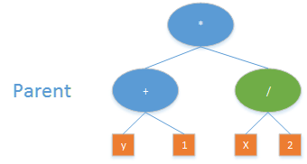
Figure 5. Genetic programming mutation
 
Reproduction simply copies the selected program intact to the next generation with no modification.

References

Keane, A. J. (1996). THE DESIGN OF A SATELLITE BOOM WITH ENHANCED VIBRATION PERFORMANCE USING GENETIC ALGORITHM TECHNIQUES. The Journal of the Acoustical Society of America, 99(4), 2599–2603.

Poli, R., Langdon, W. B., McPhee, N. F., & Koza, J. R. (2008). A field guide to genetic programming. Lulu. com.