In prior posts, I showed that genetic programming could be used to fit an expression to a set of experimental data. This technique is know as symbolic regression and is used to model the underlying data generating process (DGP) describing observed data points. A series that was easily modeled is show again below

The underlying DGP is described by the equation :

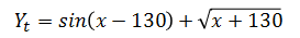
In that experiment, genetic programming did a good job of approximating this series, with a final mean error of 0.012.

But what happens if the DGP changes, either abruptly or gradually, over time? Financial series are known to exhibit this behavior. For example, the following chart of the S&P 500 before and after the financial crisis in 2008. The underlying factors before and after the crash and during the subsequent recovery are likely quite different.

S&P 500 index close price during the stock market crash of 2008 (Yahoo, 2013)

An example synthetic (made up) series that exhibits structure breaks, or regime change, is the following:

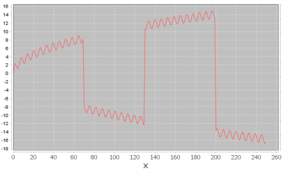
This series is represented by the equation:

Taken separately as two (or possibly four) individual series, GP would easily find the correct solution to each. But without a way to break the series up, GP does not perform very well. Using the same parameters as in the prior experiment, GP finishes the run with an average error of 1.71, compared with an average error of .01 for the (slightly more complicated) series in the prior experiment.

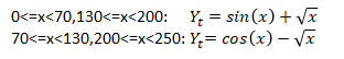
The final regression achieved is shown in the following diagram:

You can view the log of the run :

[Symbolic regression with regime change log.txt].

The video is shown below.

One easy way to improve this situation is to add autoregressive and logical functions to the primitive set. By autoregressive, I mean functions that make use of prior series values. Chaotic series are determined by such functions, but this series is not chaotic. However, adding such functions can yield much better predictions. As we know the actual DGP does not include an autoregressive term, the use of such functions will likely not indicate the actual DGP, but only an approximation. Additional logical functions are included to enable decisions that could potentially model underlying regime switching.

A risk in including autoregressive functions is that the prediction can converge early to a random walk prediction, where the predicted value is simply the prior value. One way to avoid this is to not allow expressions that evaluate to the prior value. While this may be cheating a bit for this series, autocorrelation functions are requirements for chaotic series and likely required for financial series.

The following experiment adds the following three functions to the primitive set:

• PeriodMin – minimum x value within a given prior period
• PeriodMax – maximum x value within a given prior period
• OffsetValue – value of x a given period ago.

For these three functions, the offset periods are determined through evolutionary operations.

The following logical expressions are also added:

• And  – logical And
• Not  – logical negation
• GT  – logical greater than
• LT  – logical less than
• ifElseBoolean – if else with Boolean parameters
• ifElseNumeric –if else with numeric parameters

The following run uses the same parameters as the prior run along with the inclusion of the additional primitives.

The log of the run is here:

[Symbolic regression with regime change and autoregressive functions log.txt]

and a video of the run is shown below.:

Notice the prediction immediately converges on a somewhat trivial prediction but adjusts and improves over time. The diagram below shows the results after one generation. The function shown is the equivalent of y(t)=y(t-1) +1.

The final result does a bit better, with an average error of 0.31, and is shown in the diagram below. Still, the result is not as good as what can be achieved on similar series that don’t contain structural breaks.

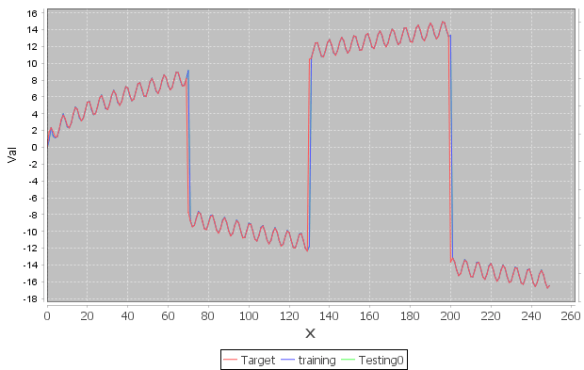
An analyst looking at this series might notice that it is broken up into either two series or four similar segments. Therefore, he might choose to run different models on each section and take each prediction individually. In fact, this is often how regime change is handled when modeling financial series*. However, forcing the analyst to choose the appropriate time window for analysis limits the potential automated solutions (Wagner et al., 2007. P.2).

An alternative approach that I developed in my PhD dissertation automatically infers regime boundaries and allows the development of distinct solutions for each regime. Using this technique, the run converges to the exact solution (ignoring some rounding errors) after 26 generations. The final (correct) solution is shown below.

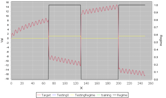
The black line shows the inferred regimes, as indicated by the right vertical axis. In this approach, different expressions are automatically generated for different regimes. Regime boundaries are determined through typical evolutionary operations.

Here is the log for this run

[Symbolic regression with regime change and automatically defined templates log.txt.

A video of the run is shown below.

I will discuss this technique, which I named “automatically defined templates”, further in future blogs. For now, you can see my PhD dissertation for additional information.

* Two econometric methods, threshold autoregressive model and the Markov regime switching model, consider regime change. Both approaches break the time series into two or more separate series, one for each regime, and apply traditional modeling techniques, such as ARMA, to each independently.

References:

Wagner, N., Michalewicz, Z., Khouja, M., & McGregor, R. R. (2007). Time Series Forecasting for Dynamic Environments: The DyFor Genetic Program Model. IEEE Transactions on Evolutionary Computation, 11(4), 433–452. doi:10.1109/TEVC.2006.882430

Yahoo. (2013). Yahoo Finance. Retrieved from http://finance.yahoo.com/